Wang Shusen Recommender Systems Study Notes — Ranking
Wang Shusen Recommender Systems Study Notes — Ranking
Ranking
Multi-Objective Ranking Model
User–Post Interactions
-
For each post, the system records:
- Number of impressions
- Number of clicks
- Number of likes
- Number of favorites
- Number of shares
-
Click-through rate (CTR) = clicks / impressions
-
Like rate = likes / clicks
-
Favorite rate = favorites / clicks
-
Share rate = shares / clicks
Basis for Ranking
- The ranking model estimates click-through rate, like rate, favorite rate, share rate, and other scores.
- Fuse these estimated scores. (e.g., weighted sum.)
- Rank and truncate based on the fused score.
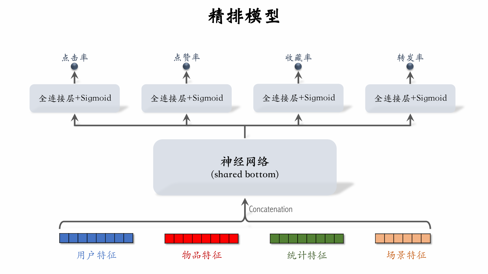
Multi-Objective Model
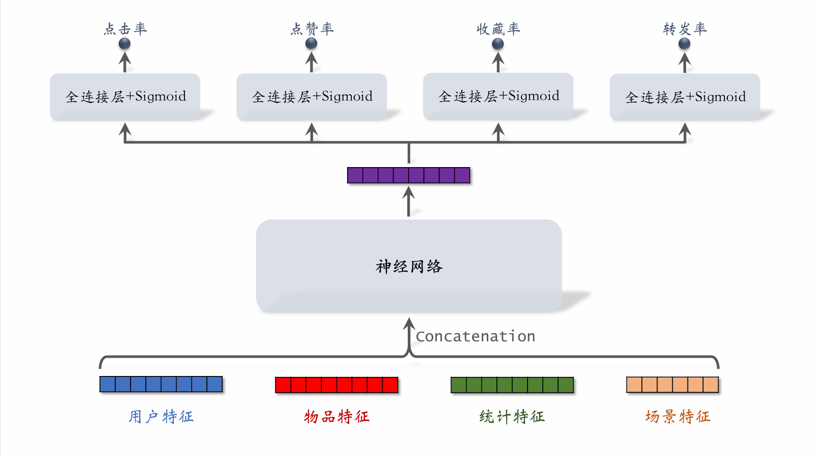
- User features: e.g., user ID, user profile
- Item features: e.g., item ID, item profile, author information
- Statistical features: e.g., how many posts a user has been exposed to, clicked, or liked over a recent time period; how many impressions, clicks, or likes an item has received over a recent time period
- Context features: e.g., current time, user's location
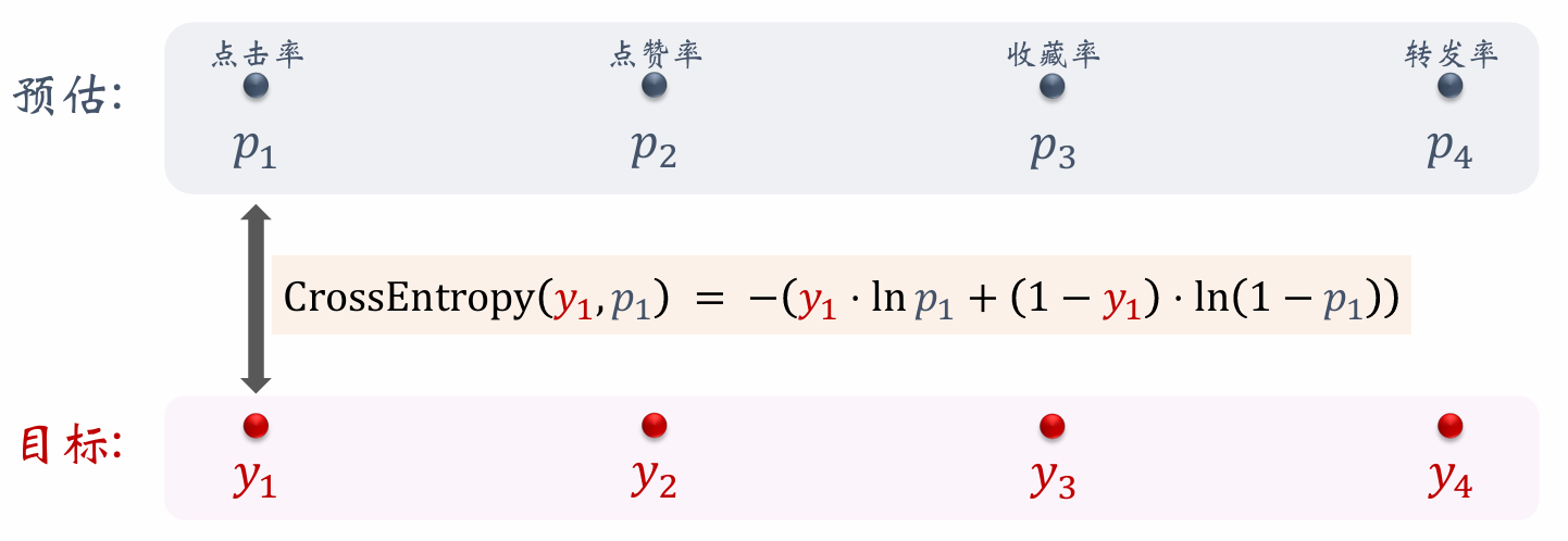
Training:
-
For click-through rate, the model essentially classifies whether an item was clicked — a binary classification problem, using cross-entropy loss.
-
Total loss function: .
-
Compute gradients of the loss function and update parameters via gradient descent.
Training
-
Challenge: Class imbalance.
- Out of every 100 impressions, approximately 10 clicks and 90 non-clicks.
- Out of every 100 clicks, approximately 10 favorites and 90 non-favorites.
- The gap between negative and positive samples is large; extra negative samples add little value and waste compute.
-
Solution: Negative sample down-sampling (down-sampling)
- Keep a small fraction of negative samples.
- Balance positive and negative sample counts to save compute.
Predicted Value Calibration
-
Let the number of positive and negative samples be and .
-
Down-sample negative samples, discarding a fraction.
-
Use negative samples, where is the sampling rate.
-
Because there are fewer negative samples, the estimated click-through rate is higher than the true click-through rate. The smaller , the fewer negative samples, and the more the model overestimates click-through rate.
-
True click-through rate:
- Estimated click-through rate:
- From the two equations above, the calibration formula is:
Multi-gate Mixture-of-Experts (MMoE)
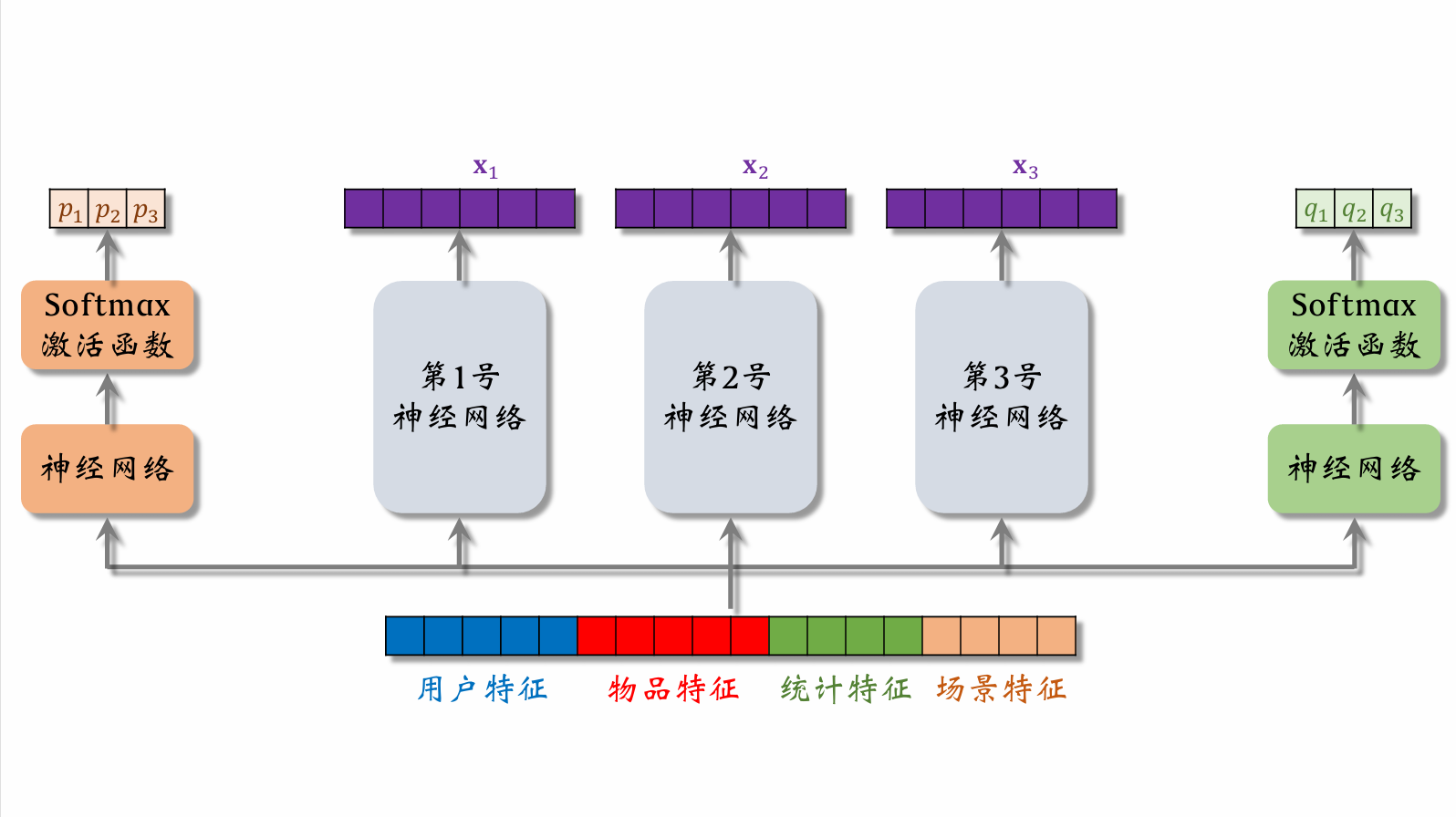
Expert networks 1, 2, and 3 are the expert neural networks.
User features, item features, statistical features, and behavior features are fed into the left neural network, then passed through a softmax activation function to produce a weight vector. This type of network is called a gating network. The three values in the vector represent the weights assigned to respectively. The right side works analogously.
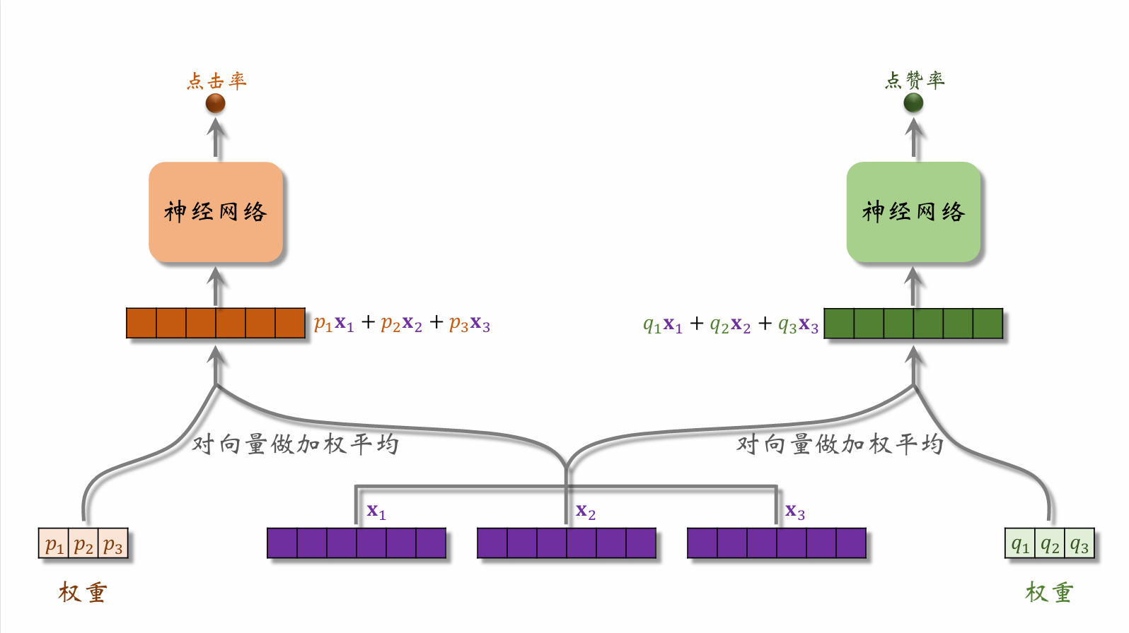
The weight vector from the left gating network is combined with the feature vectors from the expert networks and fed into the left task network to predict click-through rate. The right side works analogously.
Polarization
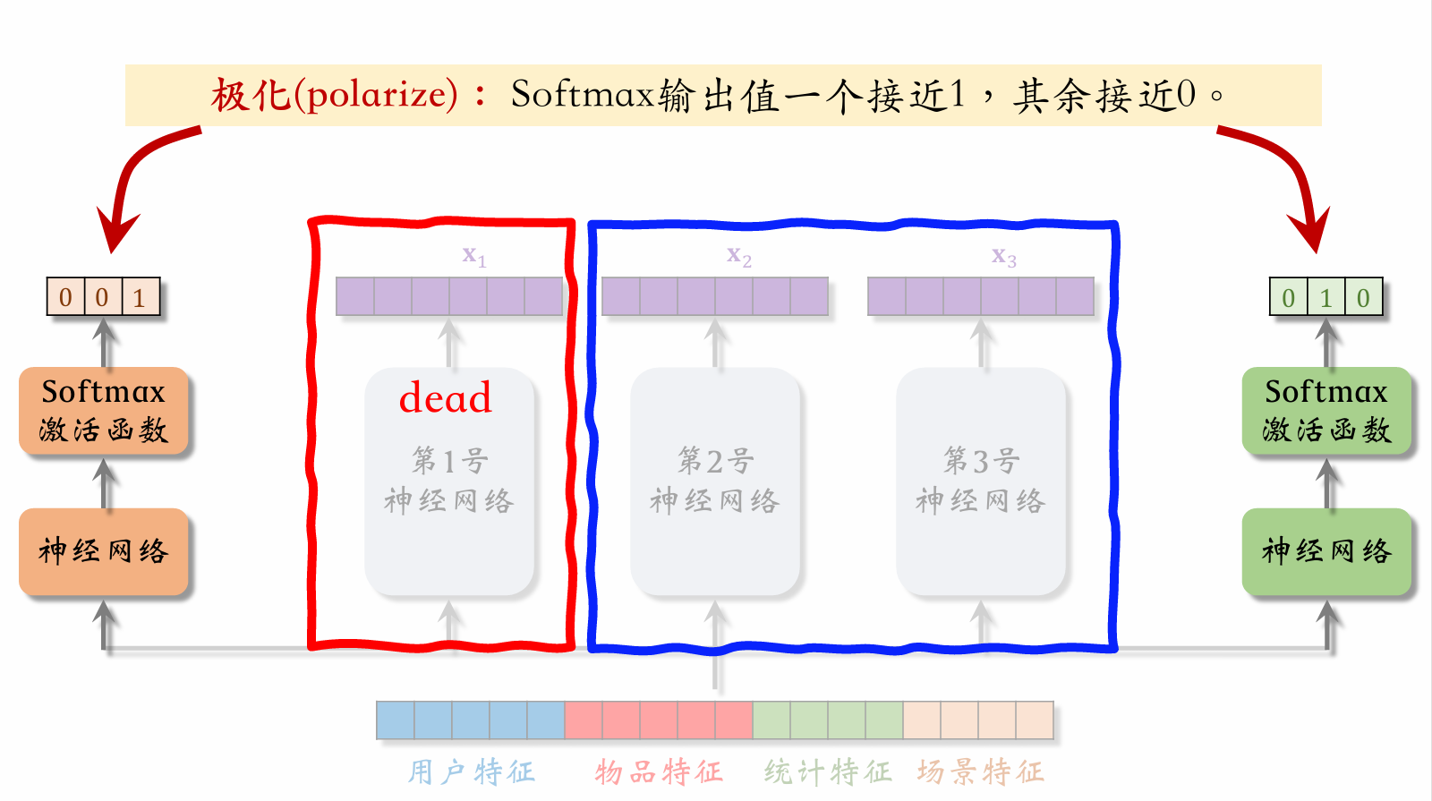
When the left gating network's weight vector assigns close-to-1 weight to expert 3 and close-to-0 weight to the others, and the right gating network's weight vector assigns close-to-1 weight to expert 2 and close-to-0 weight to the others, the result is that expert 1's output doesn't participate in the model at all. This situation should be avoided.
Addressing Polarization
-
If there are "experts," each softmax's input and output are -dimensional vectors.
-
During training, apply dropout to the softmax output:
- Each of the softmax output values is masked with 10% probability.
- Each "expert" has a 10% probability of being randomly dropped.
Score Fusion
Simple Weighted Sum
Click Rate Multiplied by Weighted Sum of Other Terms
Fusion Score Formula from a Domestic Short-Video App
- Rank candidate videos by estimated watch time .
- If a video ranks , its score is .
- Apply similar treatment to estimated scores for clicks, likes, shares, comments, etc.
- Final fused score: ( are hyperparameters)
Fusion Score Formula from an E-commerce Platform
-
E-commerce conversion funnel:
-
Model estimates: , , .
-
Final fused score: ( are hyperparameters)
Video Watch Time Modeling
Video Watch Duration
Image-text Posts vs. Videos
-
Main ranking signals for image-text posts:
Clicks, likes, favorites, shares, comments...
-
Video ranking additionally uses watch duration and completion rate.
-
Direct regression fitting of watch duration performs poorly. YouTube's duration modeling approach is recommended.
If , then .
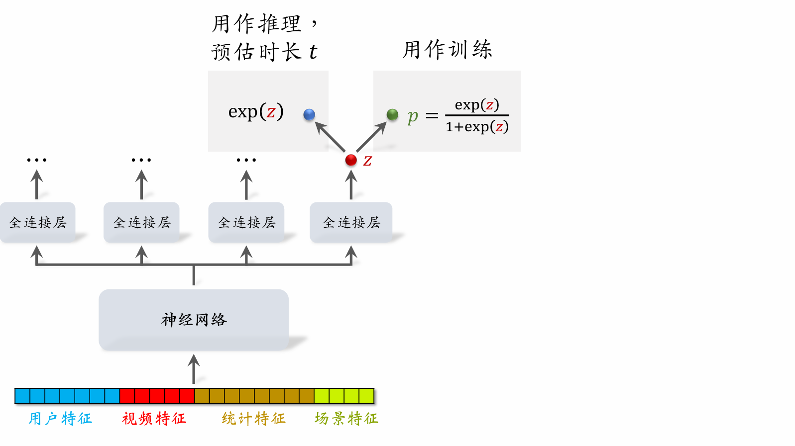
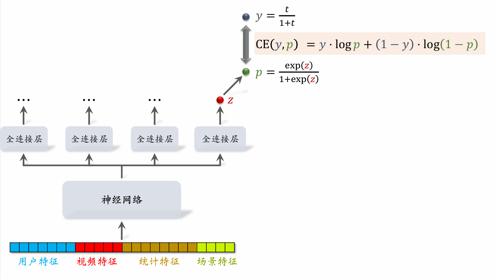
Video Watch Duration Modeling
- Let denote the output of the last fully connected layer. Set .
- Let denote the observed watch duration. (If no click, .)
- Training: minimize cross-entropy loss
- Inference: use as the estimated watch duration.
- Include as a term in the fusion formula.
Video Completion Rate
Regression Approach
-
Example: A 10-minute video was watched for 4 minutes, so the actual completion rate is .
-
Fit estimated completion rate to :
- Online estimated completion rate: model outputs , meaning an estimated 73% of the video is watched.
Binary Classification Approach
- Define a completion threshold, e.g., 80% completion.
- Example: A 10-minute video — watching >8 minutes is a positive sample; watching
<8minutes is a negative sample. - Train with binary classification: completion >80% vs. completion
<80%. - Online estimated completion rate: model outputs , meaning:
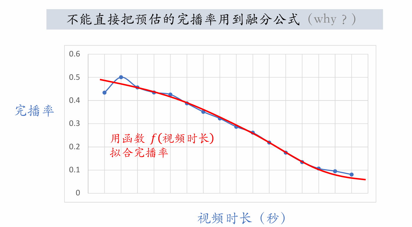
Longer videos have lower completion rates, so directly using estimated completion rate biases ranking toward short videos over long videos. Adjustment is needed to treat short and long videos fairly.
-
Online: estimate completion rate and then adjust:
-
Include as a term in the fusion formula.
Ranking Model Features
Features
User Profile
- User ID (embedded during retrieval and ranking).
- Demographic attributes: gender, age.
- Account information: new/returning, activity level...
- Categories, keywords, and brands of interest.
Item Profile
- Item ID (embedded during retrieval and ranking).
- Publication time (or age).
- GeoHash (latitude/longitude encoding), city.
- Title, category, keywords, brand...
- Word count, image count, video resolution, number of tags...
- Information richness, image aesthetics...
User Statistical Features
- Number of impressions, clicks, likes, favorites, etc. in the last 30 days (7 days, 1 day, 1 hour)...
- Bucketed by post type (image-text / video). (e.g., the user's click-through rate on image-text posts vs. video posts in the last 7 days.)
- Bucketed by post category. (e.g., the user's click-through rate on beauty posts, food posts, and tech posts in the last 30 days.)
Post Statistical Features
- Number of impressions, clicks, likes, favorites, etc. in the last 30 days (7 days, 1 day, 1 hour)...
- Bucketed by user gender, user age...
- Author features:
- Number of published posts
- Number of followers
- Consumption metrics (impressions, clicks, likes, favorites)
Context Features
- User location GeoHash (latitude/longitude encoding), city.
- Current time (discretized and embedded).
- Whether it's a weekend, whether it's a holiday.
- Phone brand, phone model, operating system.
Feature Processing
-
Discrete features: embed.
- User ID, post ID, author ID.
- Category, keywords, city, phone brand.
-
Continuous features: bucket into discrete features.
- Age, post word count, video duration.
-
Continuous features: other transformations.
- Apply to impression counts, click counts, like counts, etc.
- Convert to click-through rate, like rate, etc., and apply smoothing.
Feature Coverage
- Many features cannot achieve 100% sample coverage.
- Example: Many users don't fill in their age, so the user age feature has coverage far below 100%.
- Example: Many users set privacy permissions; the app cannot access user location, so context features are missing.
- Improving feature coverage can make the full-ranking model more accurate.
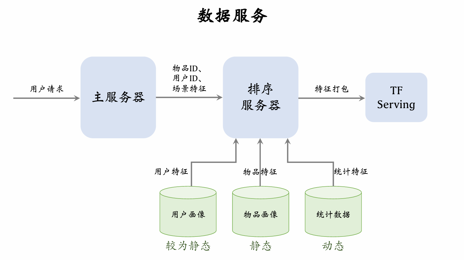
The main server retrieves a batch of item IDs from the retrieval server. The user sends a request, and the main server forwards the user ID, context features, and item IDs to the ranking server.
User profile database has lower load, since only one user's features are read per request. Item profile database has higher load, since thousands of posts' features must be read per request. Similarly, user statistics database has lower load, while item statistics database has higher load. User profile vectors can be large, but item profile vectors should not be too large.
Both user profiles and item profiles are relatively static and can even be cached locally on the ranking server. Statistical data is dynamic and requires timely database updates.
After receiving features, the ranking server packages them and passes them to TF Serving. TF scores the posts and returns results to the ranking server. The ranking server applies a series of rules to rank the posts and returns the top-ranked posts to the server.
Pre-Ranking
Pre-Ranking vs. Full Ranking
| Pre-Ranking | Full Ranking |
|---|---|
| Scores thousands of posts. | Scores hundreds of posts. |
| Per-inference cost must be low. | Per-inference cost is high. |
| Accuracy is lower. | Accuracy is higher. |
Full-Ranking Model & Two-Tower Model
Full-Ranking Model
- Early fusion: concatenate all features first, then feed into neural network.
- High online inference cost: if there are candidate posts, the large model must run inferences.
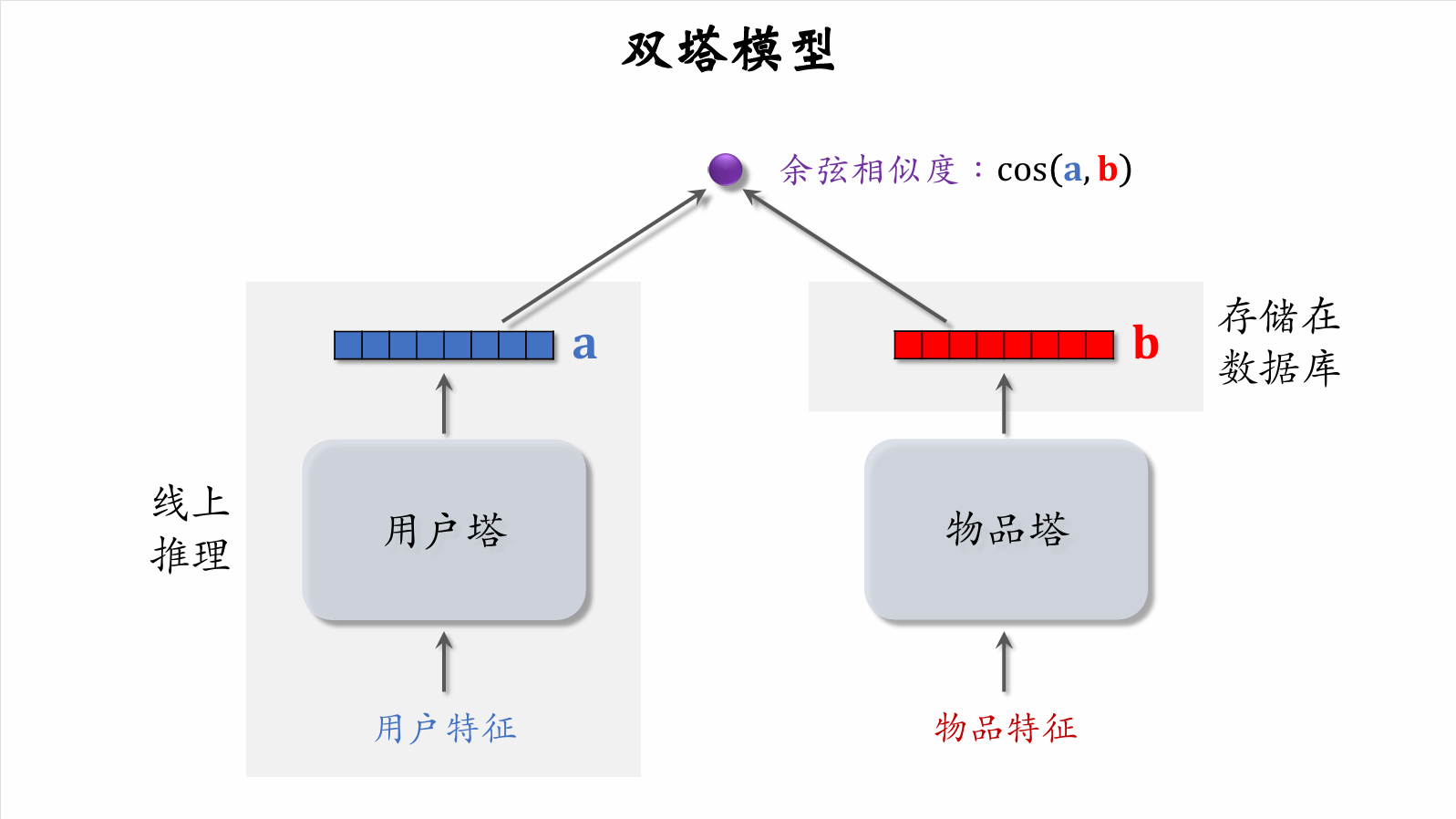
Two-Tower Model
-
Late fusion: feed user and item features into separate neural networks without fusing user and item features.
-
Low online computation:
- User tower only needs one online inference to compute user representation .
- Item representation is pre-stored in a vector database; item tower does no online inference.
-
Accuracy is lower than full-ranking model. Late fusion is less accurate than early fusion.
Three-Tower Model for Pre-Ranking
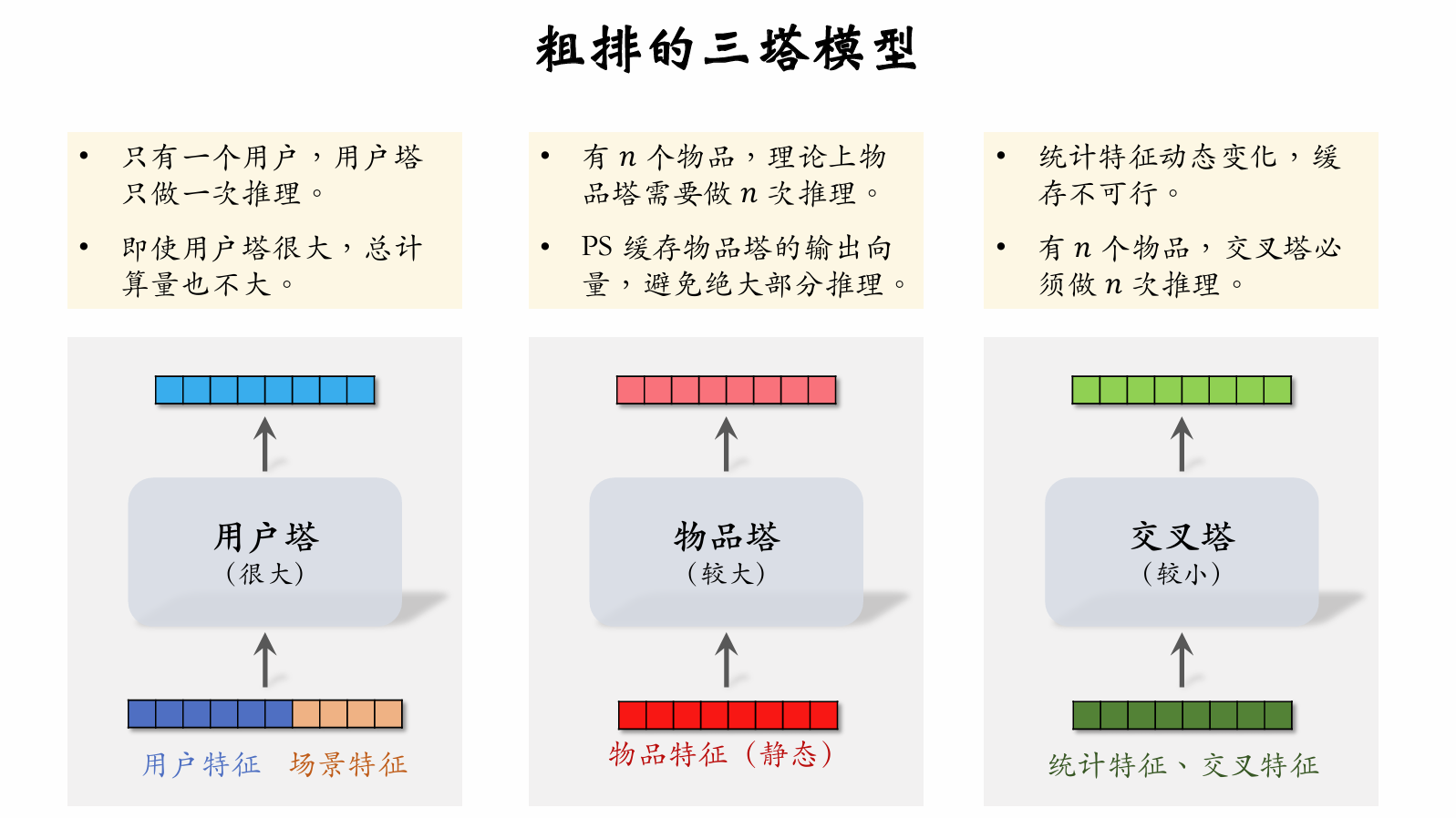
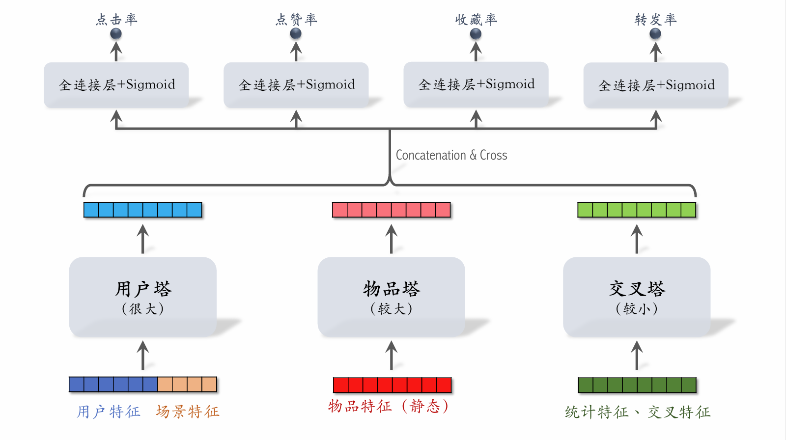
- With items, the upper model layers require inferences.
- The majority of pre-ranking computation is in the upper model layers.
Three-Tower Model Inference
-
Retrieve features from multiple data sources:
- 1 user's profile and statistical features.
- items' profiles and statistical features.
-
User tower: runs only 1 inference.
-
Item tower: runs inference only on cache misses.
-
Cross tower: must run inferences.
-
Upper network: runs inferences to score items.
贡献者
最近更新
Involution Hell© 2026 byCommunityunderCC BY-NC-SA 4.0![]()
![]()
![]()
![]()